Statistics in Archaeology

Thomas Huet (University of Oxford, EAMENA project)

Introduction
Grémy et Salmon, 1967
“Le but de la statistique est d’étudier un certain nombre d’objets de même nature, mais qui présentent des caractéristiques variables susceptibles de mesure ou de classement”


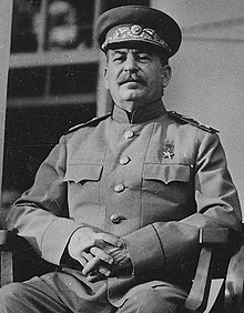
Joseph Staline, 1953
“Смерть одного человека — трагедия, смерть миллионов — статистика”


Winston Churchill, 1941
“the only statistics you can trust are the ones you have falsified yourself”

Inequalities

Historiography of Archaeology 1/2

Start Method Description
1850s Prehistory evolution, geology, anthropology
1950s Culture-Historical similarities, typology, chronology
1960s New archaeology chain operative, statistics, chronology (C14)
1980s Post-processual dissimilarities, cultural relativism
2020s Tool-driven Big data, ML / DL, aDNA
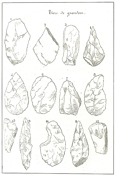
Boucher de Perthes, 1847, Antiquités celtiques et antédiluviennes
Concomitance between biological “species” (C. Darwin) and archaeological “types” (O. Montelius). Unity of the history of Nature with that of Man (C. Lyell, geology)
‘Monument druidique près de Gisors’: Baron Taylor, 1824, Voyages pittoresques et romantiques dans l’ancienne France
Focused on chronology, rooted in academic/national traditions and develops in parallel with History as a ‘scientific’ discipline taught in universities.

Historiography of Archaeology 2/2


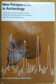
R. & S. Binford, 1968, New Perspectives in Archaeology
Processualism, the advancement of statistics favors demonstrations based on observations, hypotheses, models and tests. With the development of anthropology, archaeology focuses on the recent past. Chronologies have an anthropological and explanatory purpose.
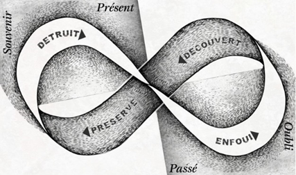
Laurent Olivier, 2008, Le sombre abîme du temps
Post-processualism1, archaeology adopts a qualitative point of view and insists on the importance of context and the variability of possible interpretations (relativism, multivocity)
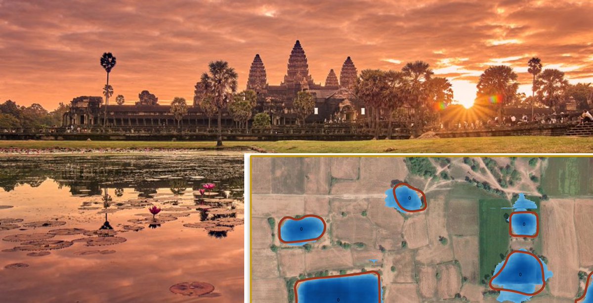
Automatic detection of water basins in Angkor Bath with ML/AI, by Jürgen Landauer

With the development of computational archaeology (e.g. AI/ML, aDNA) and oceans of data, the archaeologist becomes a research software engineer. A single project probably cannot exploit the full potential of the data at hand. Data is managed and made FAIR2 to produce serendipity over the long term.

Birth of statistics
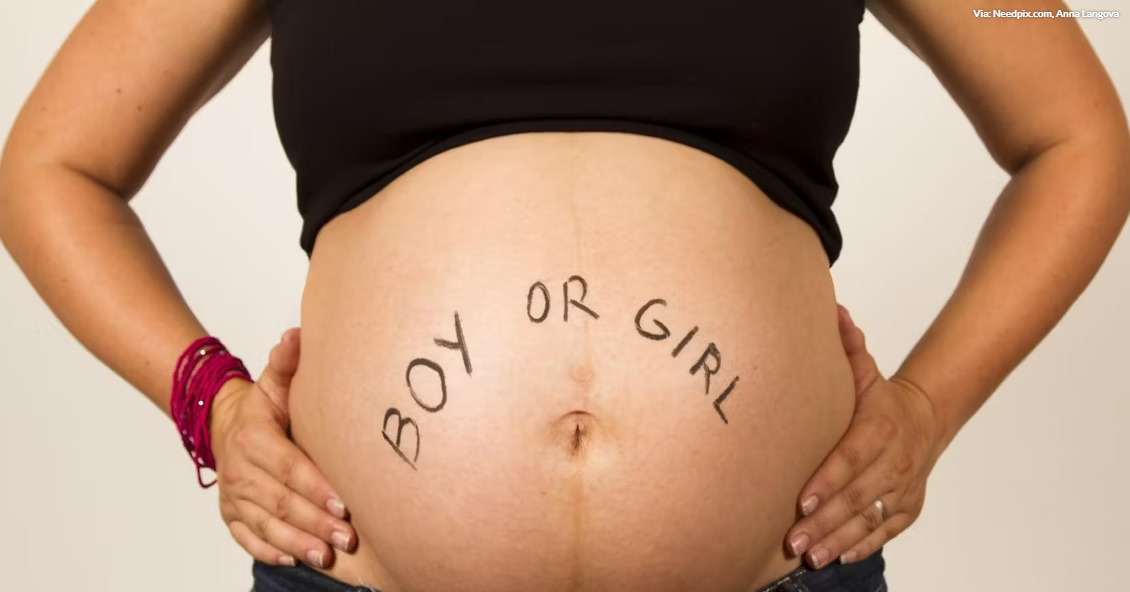
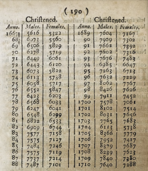
Sex ratio at birth
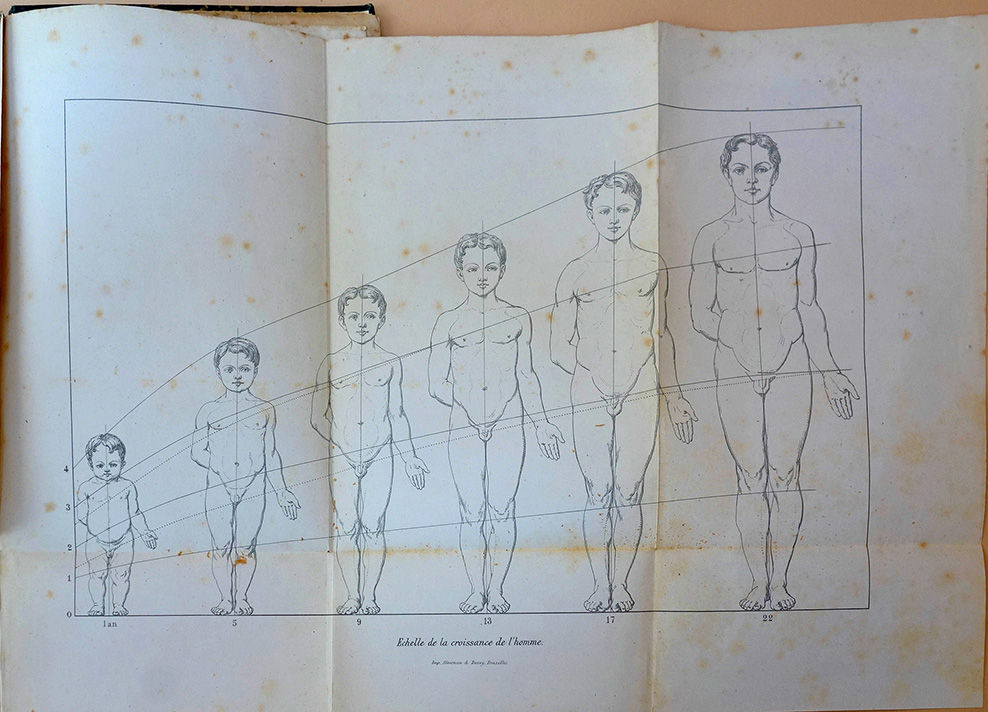
“Anthropométrie ou mesure des différentes facultés de l’homme”, 1870, by A. Quetelet
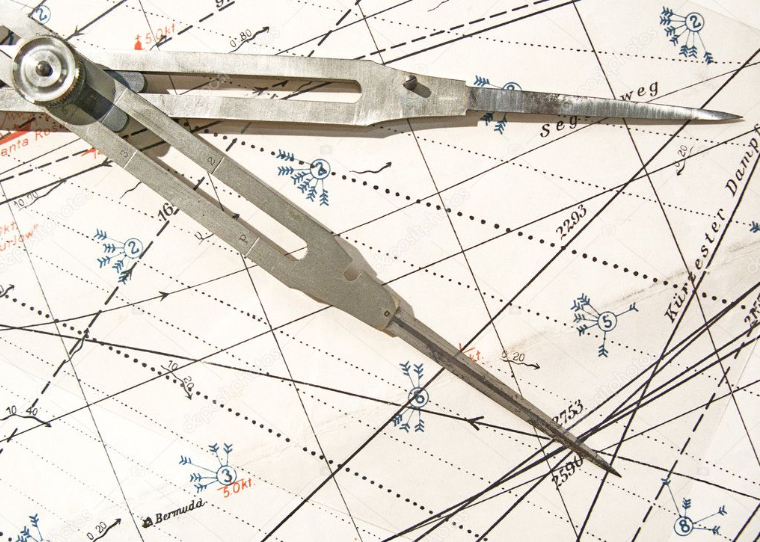
Title page of E. Wright, 1599, ‘Certaine Errors in Navigation’
J. Arbuthnott, 1629-1710 census. Published in 1711, ‘Philosophical transactions, 27’
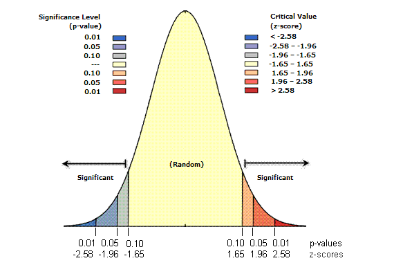
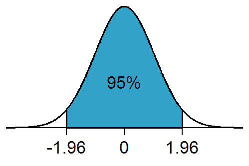
p-value and Z-score, two normalised test thresholds to estimate the significance of an observed distribution vs a random distribution


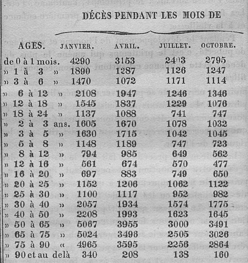
A. Quetelet, 1821-1833 census
A selection of Normal Distribution Probability Density Functions

Advanced statistics

Garry Kasparov vs Deep Blue, 1996-1997
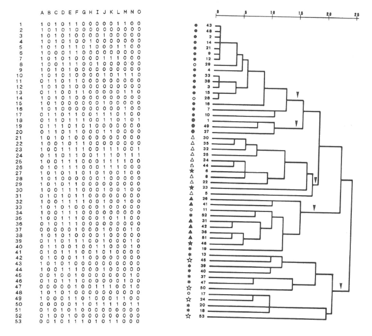
Hierachical clustering of the Iberian LBA “Warrior stelae”, Galàn 1993

Artificial Intelligence & Machine Learning

Natural language processing (NLP), prompted by ChatGPT, 2023
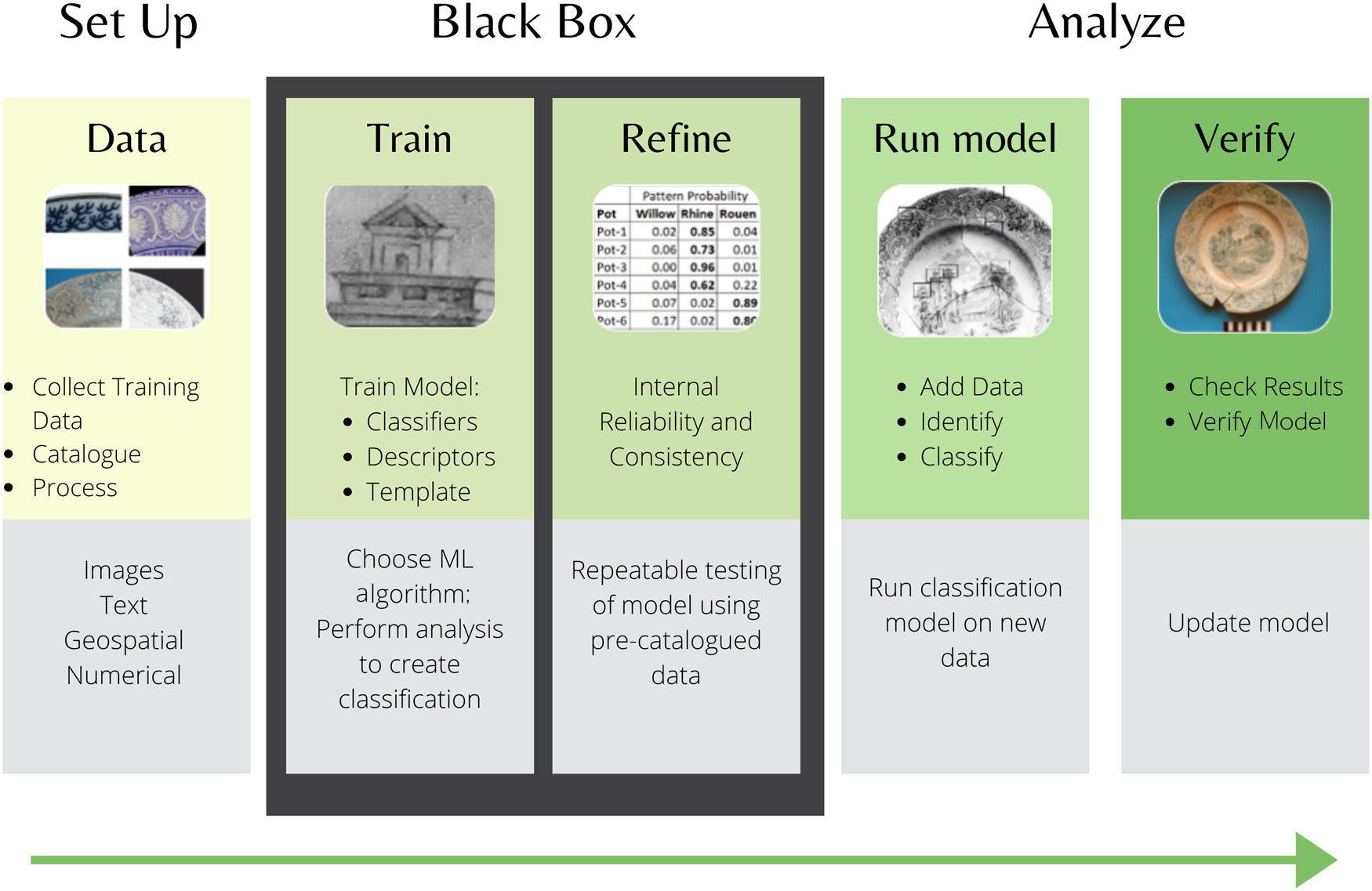
Example of ML workflow applied to ceramics, S.H. Bickler, 2021

Glossary of statistics

Type of statistics
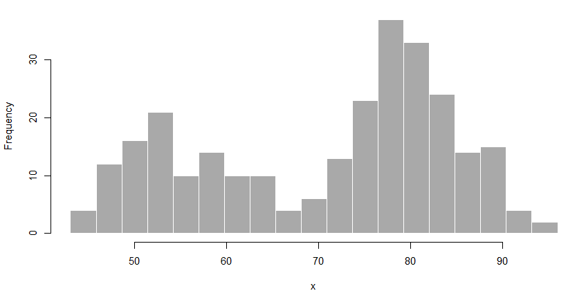
Descriptive

Explanatory

Confirmatory

Describe the population with the mean (μ), the median (M) and standard deviation (σ)
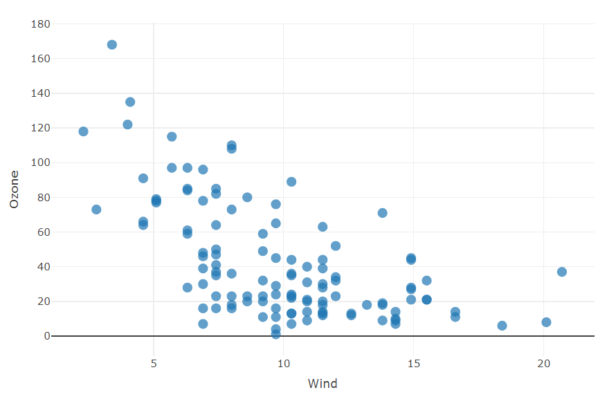
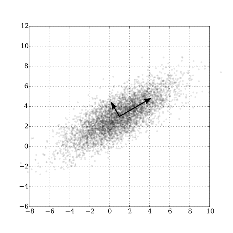
Scatterplot

Histogram

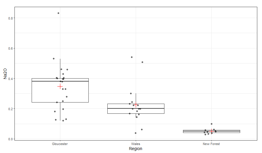
Boxplot

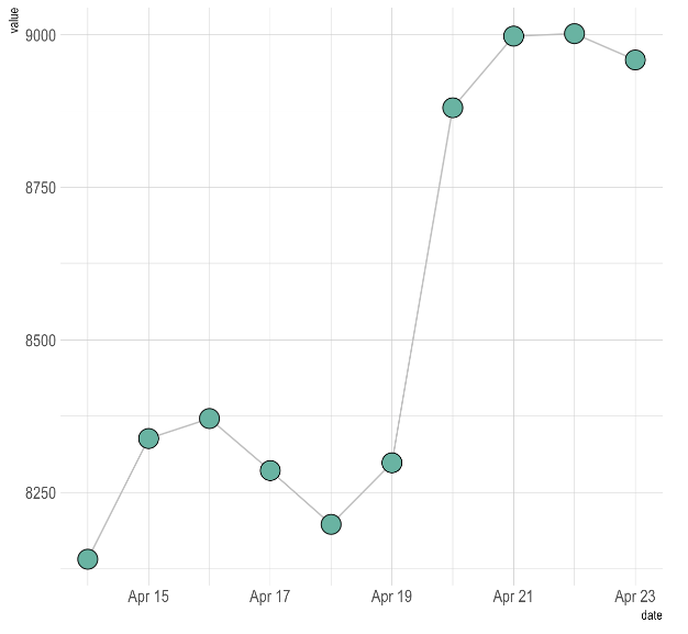
Line chart

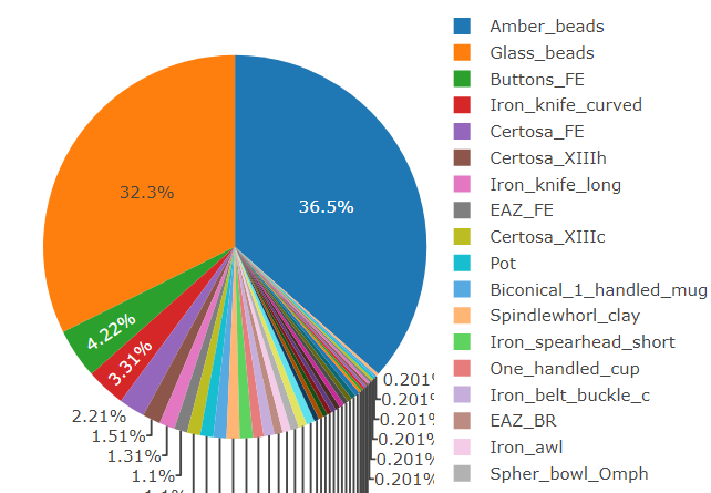
Pie Chart

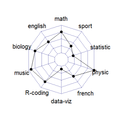
Radar chart

Clustering method, we move from a description to a modelling identifying central tendencies
Test of
  • conformity3 between the observed population and a theoretical distribution (e.g. normal law)
  • homogeneity between different populations
  • relation between several variables from the same population

Middle Range Theories

Archaeology establishes facts and proposes models to connect these facts
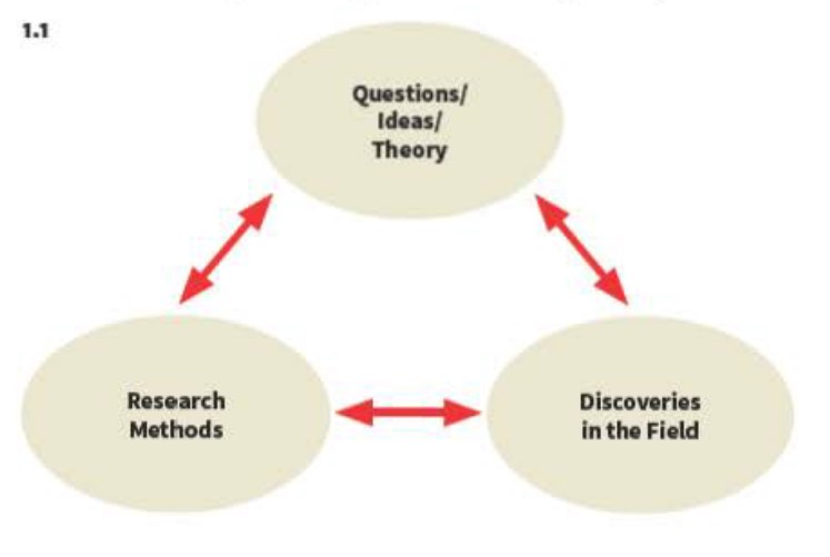
Model of archaeological reasoning by Renfrew and Bahn, 2020
“Sociological theory, if it is to advance significantly, must proceed on these interconnected planes”4
Robert K. Merton, 1968

We want to compare 3 different archaeological cultures5 (groups of settlements, sites, geographical regions, chronological periods, etc.): A, B, and C
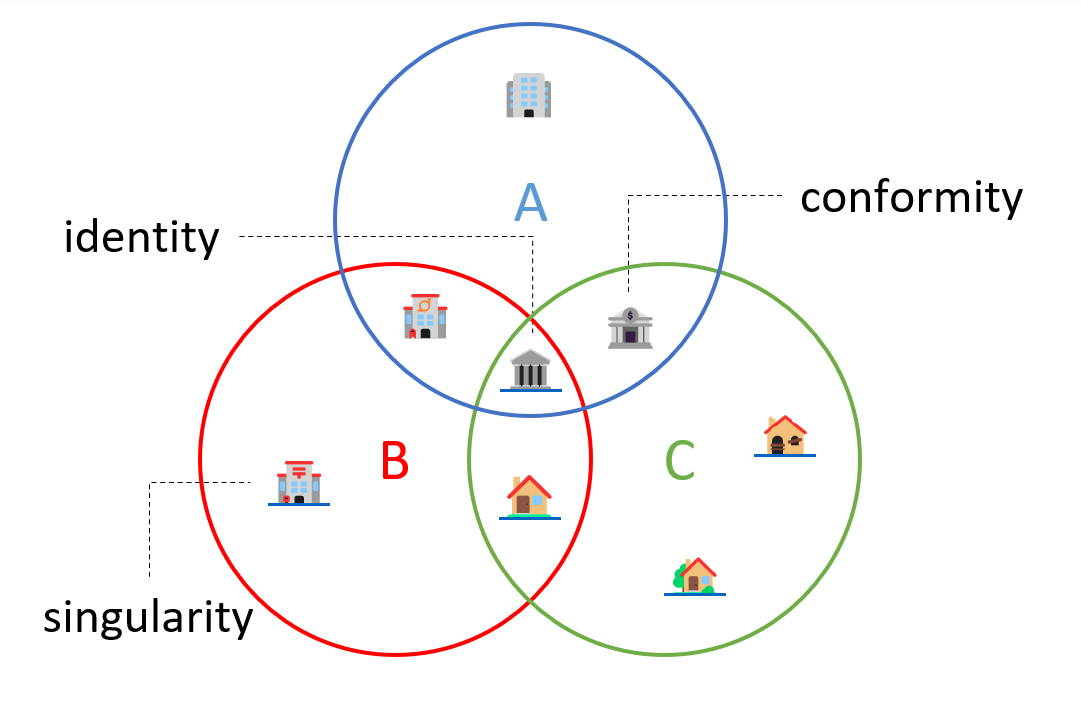
None of the comparisons gives the same results
⚠️ In practice, over-valuing a specific element by giving it a marker character is dangerous, as its originality makes its management uncontrollable.
Most comparisons give the same results
💡 Increase the matching success of the model by decreasing its precision, or decrease the matching success of the model by increasing its precision.
All the comparison give the same result
⚠️️In practice, a common element in 3 or more different data sets is usually rare.

Entities

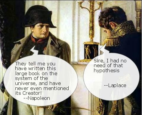
Waldo Tobler
“everything is related to everything else, but near things are more related than distant things”
Tobler, 1970
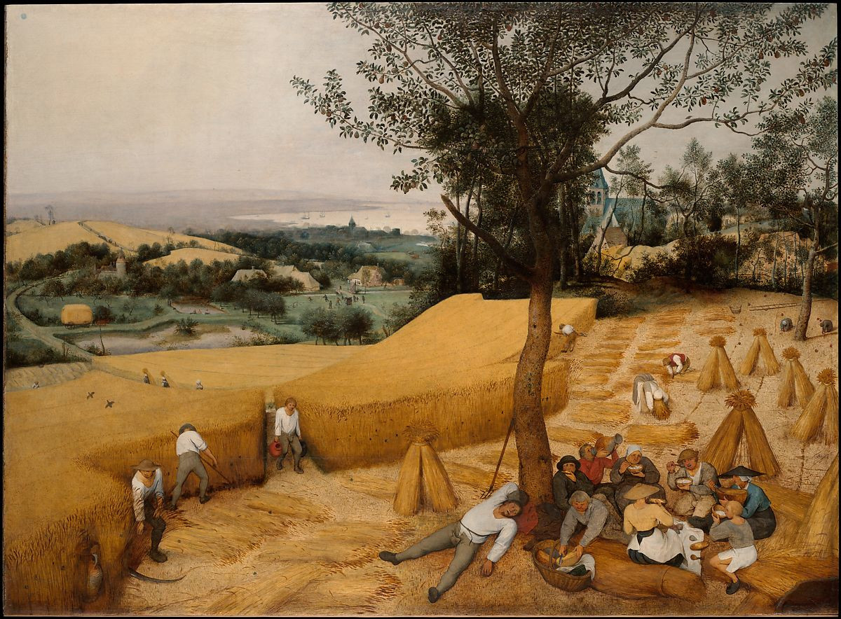
Pieter Bruegel the Elder, The Harversters, 1565
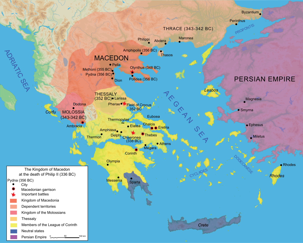
Kingdom of Macedon at the death of Philip II, 336 BC
Spiral of geological times
Startigraphic log and corresponding Harris matrix
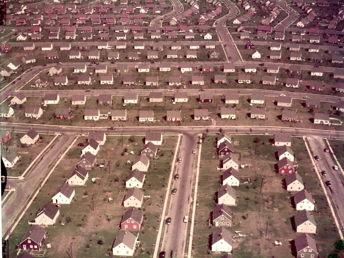
An American suburb in the 1950s

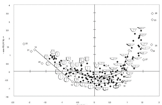
Seriation of Chassean potteries in South France
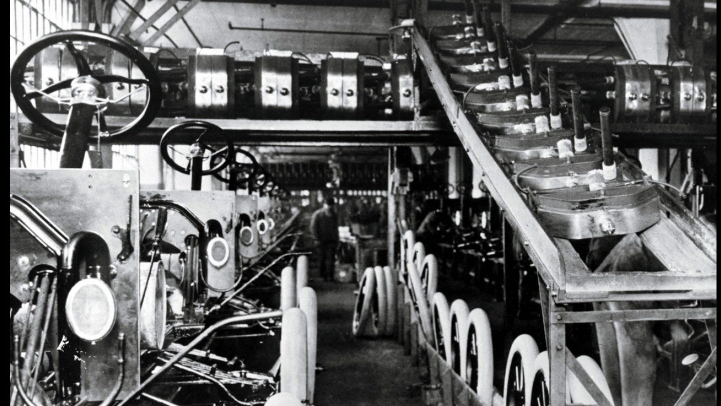
Assembly line work in a Ford factory
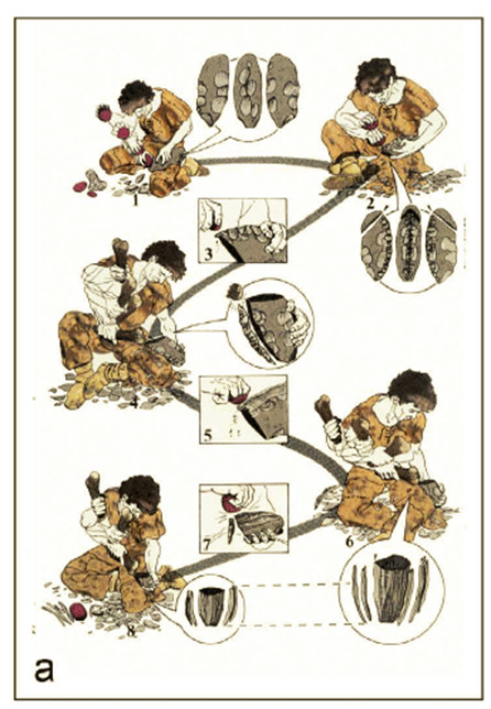
Chaine opératoire of flint lamellas knapping
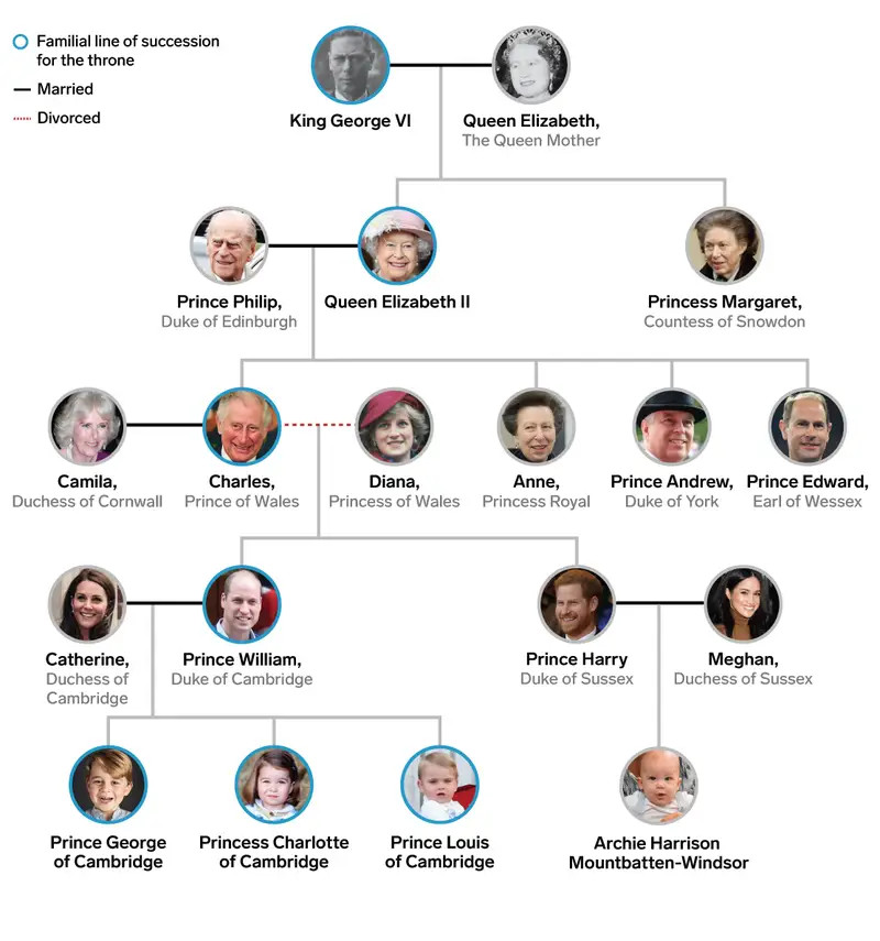
The British Royal Family6
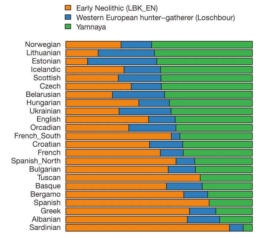
Estimate DNA mixture proportions of Modern Europeans

Conformity


⬇️ distance matrix
A B C
A 0.00 3.24 2.53
B 3.24 0.00 1.05
C 2.53 1.05 0.00


Khi-square

χ 2


  • Observed numbers
Code
library(dplyr)
library(tibble)

df <- data.frame(patient = c("Mal.1", "Mal.2", "Mal.3"),
                 virus.A = c(12, 19, 13),
                 virus.B = c(7, 7, 10),
                 virus.C = c(11, 4, 5))
kable(df) %>%
  kable_styling(full_width = FALSE, position = "center", font_size = 24)
patient virus.A virus.B virus.C
Mal.1 12 7 11
Mal.2 19 7 4
Mal.3 13 10 5

  • Calculation of rows and columns sums
Code
df.copy <- df
df.copy <- rbind(df.copy, colSums(df.copy[ , -1]))
df.copy[nrow(df.copy), "patient"] <- "col.sum"
df.copy <- cbind(df.copy, rowSums(df.copy[ , -1]))
colnames(df.copy)[ncol(df.copy)] <- "row.sum"
kable(df.copy) %>%
  kable_styling(full_width = FALSE, position = "center", font_size = 24) %>%
  column_spec(ncol(df.copy), bold = TRUE) %>%
  row_spec(nrow(df.copy), bold = TRUE)
patient virus.A virus.B virus.C row.sum
Mal.1 12 7 11 30
Mal.2 19 7 4 30
Mal.3 13 10 5 28
col.sum 24 20 44 88

  • Calculation of expected numbers (E)
Code
chisq <- chisq.test(df[ , -1])
df.copy2 <- as.data.frame(round(chisq$expected, 2))
df.copy2$patient <- df$patient
kable(df.copy2) %>%
  kable_styling(full_width = FALSE, position = "center", font_size = 24)
virus.A virus.B virus.C patient
15 8.18 6.82 Mal.1
15 8.18 6.82 Mal.2
14 7.64 6.36 Mal.3

  • Differences between expected (E) and observed (O) numbers
Code
df.copy3 <- as.data.frame(round(chisq$residuals, 2))
df.copy3$patient <- df$patient
kable(df.copy3) %>%
  kable_styling(full_width = FALSE, position = "center", font_size = 24)
virus.A virus.B virus.C patient
-0.77 -0.41 1.60 Mal.1
1.03 -0.41 -1.08 Mal.2
-0.27 0.86 -0.54 Mal.3


  • Khi-2 calculation
Code
khi2.df <- matrix(nrow = length(df$patient),
                                ncol = length(df$patient))
colnames(khi2.df) <- rownames(khi2.df) <- df$patient
khi2.df[1 , 2] <- round(chisq.test(df[, c(2, 3)])$p.value, 2)
khi2.df[2 , 1] <- round(chisq.test(df[, c(2, 3)])$p.value, 2)
khi2.df[1 , 3] <- round(chisq.test(df[, c(2, 4)])$p.value, 2)
khi2.df[3 , 1] <- round(chisq.test(df[, c(2, 4)])$p.value, 2)
khi2.df[2 , 3] <- round(chisq.test(df[, c(3, 4)])$p.value, 2)
khi2.df[3 , 2] <- round(chisq.test(df[, c(3, 4)])$p.value, 2)
khi2.df <- as.data.frame(khi2.df)
color.me <- which(khi2.df < .1)
kable(khi2.df) %>%
  kable_styling(full_width = FALSE, position = "center", font_size = 24) %>%
  column_spec(1, bold = TRUE)
Mal.1 Mal.2 Mal.3
Mal.1 NA 0.47 0.08
Mal.2 0.47 NA 0.22
Mal.3 0.08 0.22 NA


p-value and Z-score, two normalised test thresholds to estimate the significance of an observed distribution vs a random distribution

H0: ✔️ accept homogeneity hypothesis
H1: ❌ reject homogeneity hypothesis


Coefficient


cor interpretation
1
0.9 oustanding
0.8 excellent
0.7 acceptable
0.6 weak
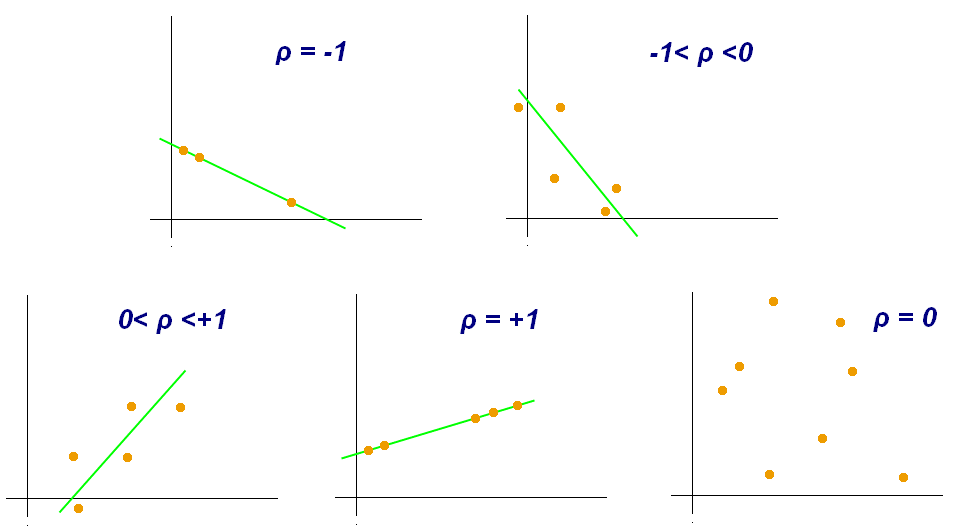
All are between [-1:1]
Coefficient of correlation
Coefficient of determination: R2

Models

George E. P. Box
“All models are wrong, but some are useful”
Box, 1976
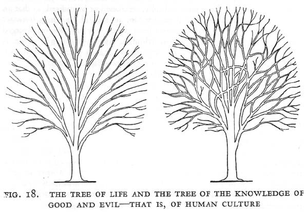
Kroeber, A. L., 1923, Anthropology: culture patterns & processes
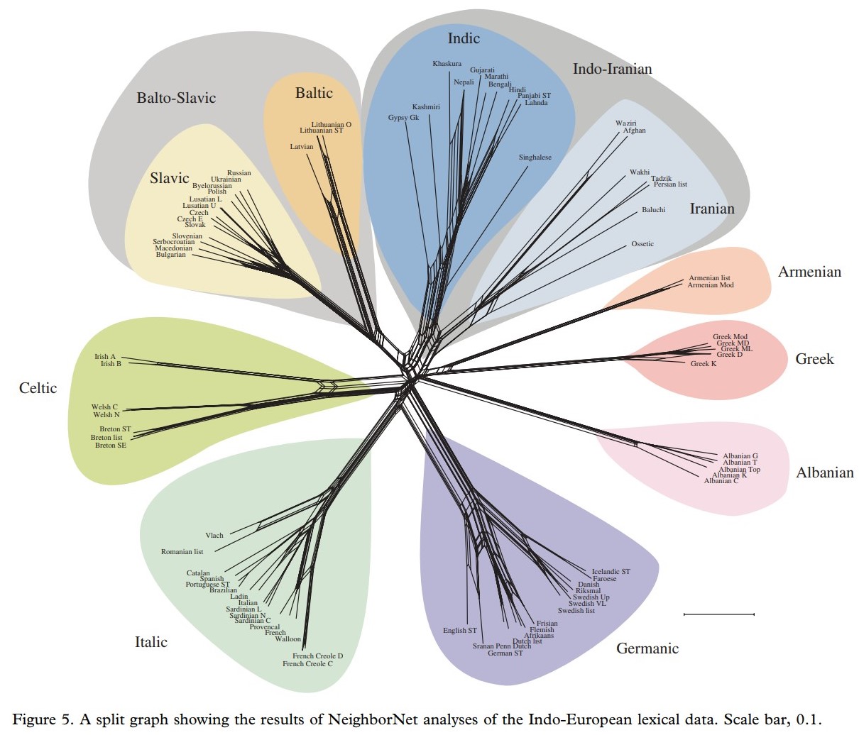
Gray, R. D., Bryant, D., & Greenhill, S. J., 2010, On the shape and fabric of human history. Philos. Trans. R. Soc. B, 365(1559), 3923-3933
propriety description example
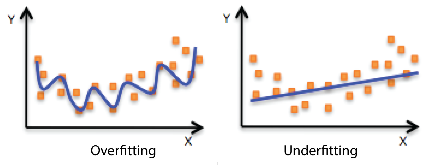
Explanatory not over- or under-fitting
Regularity reproducing data regularity
Robustness not sensitive to small changes in data
Parsimony the simplest possible explanation is also the most probable
Versioning carry its own story

Models - Proprieties

not over- or under-fitting
✔️ Fitting
❌ Fitting
reproducing data regularity (central tendencies)
not sensitive to small changes in data (reproducible)
all things being equal, the simplest possible explanation for a phenomenon is also the most probable
carry its own story: abandoned assumptions, alternative versions, etc.

Data

Raw data - Primary data acquired via a device


Processed data - Working data (i.e. not definitive)

Aggregated data - Gathered data expressed in a summary form

Metadata - data about data
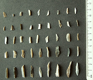
Code
img <- exiftoolr::exif_read("C:/Rprojects/thomashuet/teach/stats/images/data-meta-photo-microliths.jpg")
print(paste0("Caption-Abstract: ", img[["Caption-Abstract"]]))
[1] "Caption-Abstract: Microliths (narrow blade type): Conistone Moor (Late Mesolithic c. 6000 BC) "
Code
print(paste0("Copyright: ", img[["Copyright"]]))
[1] "Copyright: The Yorkshire Archaeological & Historical Society"


Missing data - Lack of knowledge, e.g. NA (Not Available)

Code
df <- data.frame(row.names = c("site_A", "site_B", "site_C", "site_D"),
                 Microliths =  c(10, 5, NA, 2),
                 Scrapers =  c(7, 6, 10, 5),
                 Burins =  c(13, 7, 4, NA))
kable(df) %>%
  kable_styling(full_width = FALSE, position = "center", font_size = 24)
Microliths Scrapers Burins
site_A 10 7 13
site_B 5 6 7
site_C NA 10 4
site_D 2 5 NA

Sums by column (with NA)

Code
sum.df.with.na <- as.data.frame(t(colSums(df)))
kable(sum.df.with.na) %>%
  kable_styling(full_width = FALSE, position = "center", font_size = 24)
Microliths Scrapers Burins
NA 28 NA

Sums by column (without NA)

Code
sum.df.with.na <- as.data.frame(t(colSums(df, na.rm = T)))
kable(sum.df.with.na) %>%
  kable_styling(full_width = FALSE, position = "center", font_size = 24)
Microliths Scrapers Burins
17 28 24


Boolean operators

TRUE | TRUE
[1] TRUE


TRUE | FALSE
[1] TRUE


TRUE | NA
[1] TRUE


FALSE | NA
[1] NA


TRUE & TRUE
[1] TRUE


TRUE & FALSE
[1] FALSE


TRUE & NA
[1] NA


FALSE & NA
[1] FALSE


!TRUE
[1] FALSE


!FALSE
[1] TRUE


!NA
[1] NA


Binary Topological Relationships

Kingdom of Macedon at the death of Philip II, 336 BC
Interval Temporal Logic, Allen, 1984
Central and North-Western Mediterranean Impressed Wares chronologies, 2022, Binder et al.

Scales

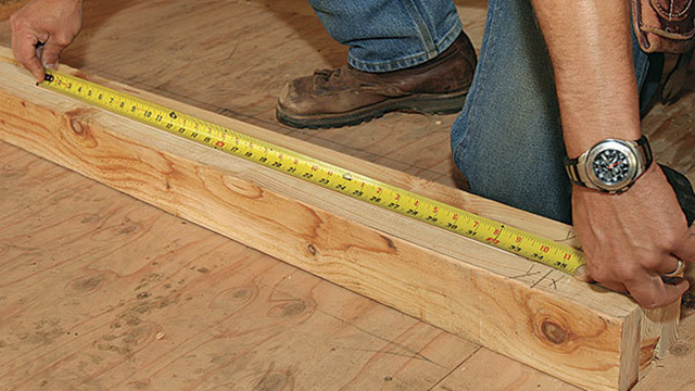
Units of length (cm, m, km, kg, years, etc.). Statistical units are quantified by continuous measurable intervals.
Ranks (discrete). Ordered sequence of values (e.g. ‘very cold’, ‘cold’, ‘lukewarm’, ‘hot’, ‘very hot’) without establishing the distance between consecutive values.
Qualitative categories that cannot be ordered (e.g. ‘green’, ‘yellow’, ‘red’).
from to transformation example
Quantitative Ordinal discretization [1:10], [11:20], etc.
Ordinal Quantitative as.numeric() "low" = 1, "medium" = 2
Ordinal Nominal as.factor()

Quantitative

Ordinal

Nominal


1-dim data

2-dim data

2-dim data spatial 1/3

2-dim data spatial 2/3

Average Nearest Neighbor Index (NNI)

NNI z.score p.value expect.mean.dist observ.mean.dist
random 1.69 5.91 0 0.85 1.43
cluster 1.64 5.51 0 0.39 0.64
regular 2.67 12.75 0 0.84 2.24


2-dim data spatial 3/3

Random patterns versus Clustered patterns
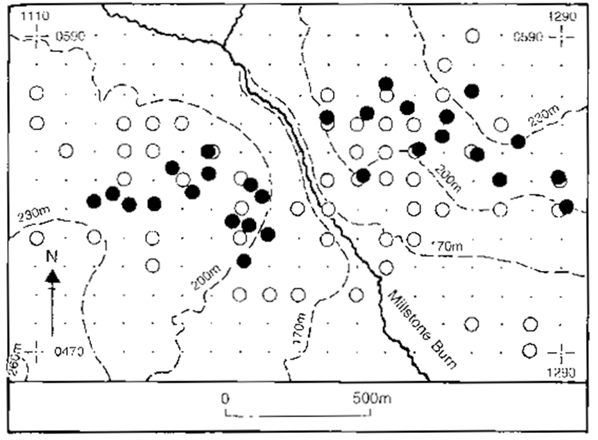
Cups-and-rings rock art concentration (⬤) in Millestone Burn, Northumberland, England (Bradley 1996)
Engraved rock sites (⬤) are concentrated on Millstone Grits (sandstone) with a statistical significance in comparison to a theoretical random distribution (○).
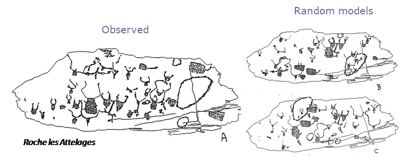
Neolithic/Early Bronze Age engraved rock, Mont Bego, France (Chippindale 1988)
On the observed rock surface (A), engravings are arranged in a more orderly manner in a random process (B and C), but the former remains far from an orderly arrangement without overlapping engravings.
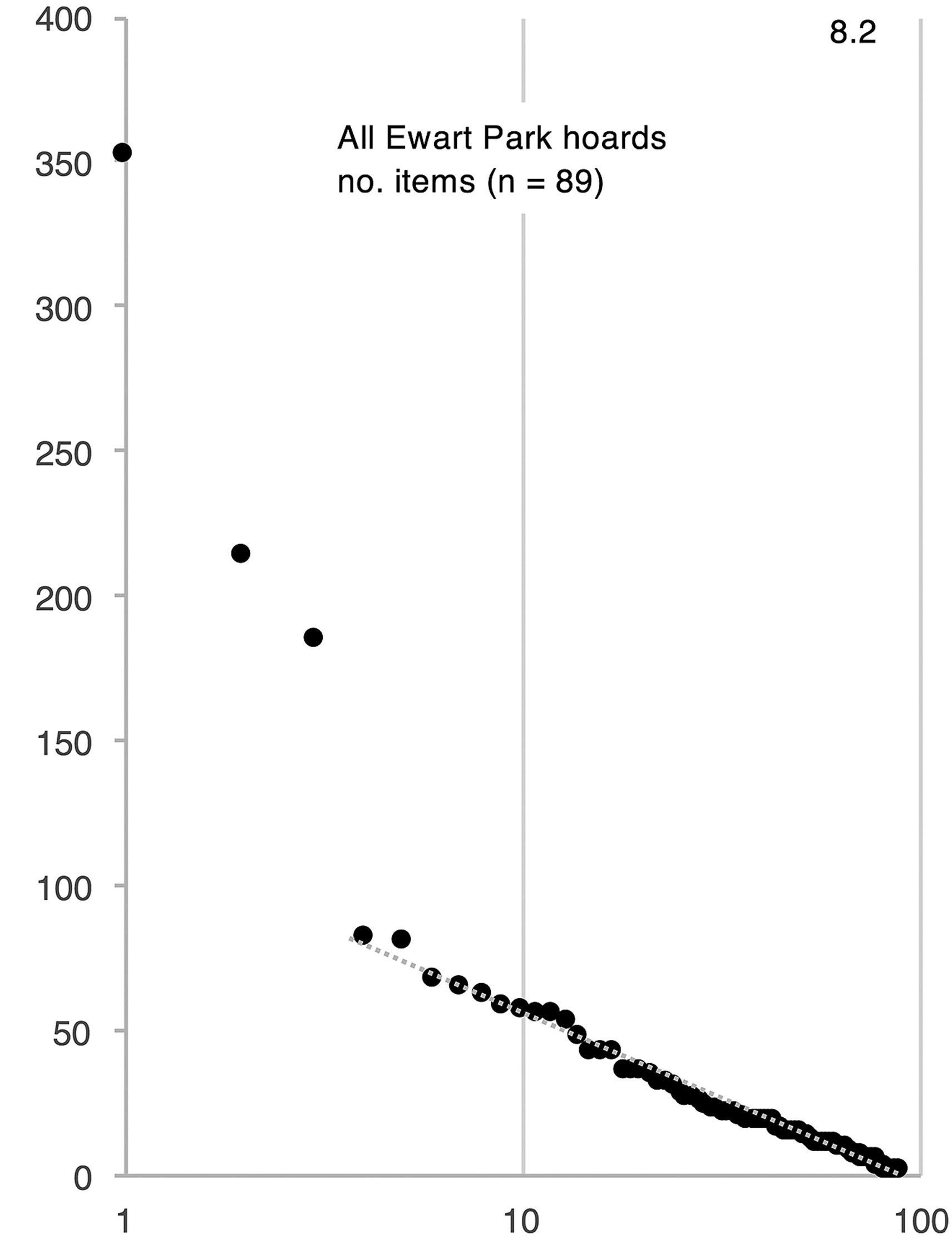
Distribution of the Late Bronze Age Ewart Park hoards, Atlantic Europe (Wiseman 2018)
Hoards from the Ewart Park phase show a normal distribution when considering size, fragmentation and number of pieces. The hoards would result from a random accumulation and breaking

Regular pattern

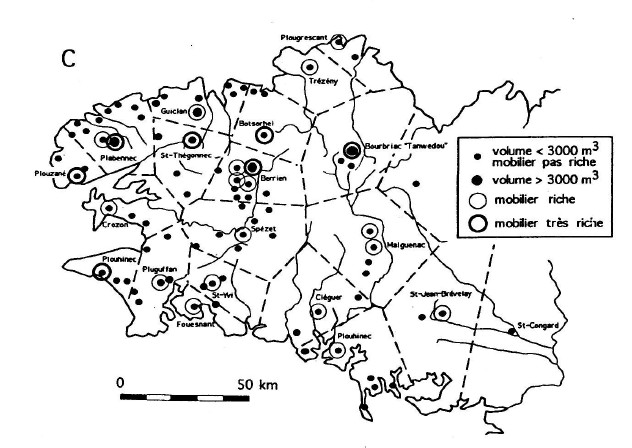
Early Bronze Age tumuli in Brittany (Brun 2011)
The ‘princely’ tombs are evenly distributed in space, separated from each other by a distance of 12.5 km, i.e. less than three hours’ walk round trip
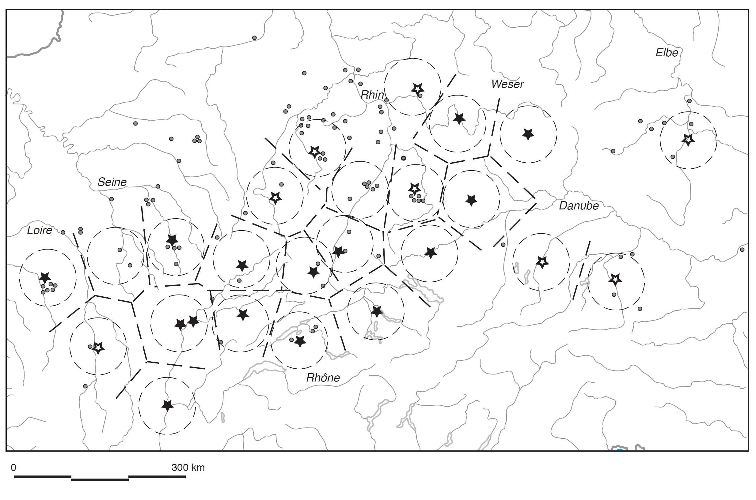
Early Iron Age princely sites at the North of the Alps (Brun 2011)
In the 6th century BC, the ‘princely sites’ are separated from each other by an average distance of about 50 km. This distance can be covered in a day on horseback.
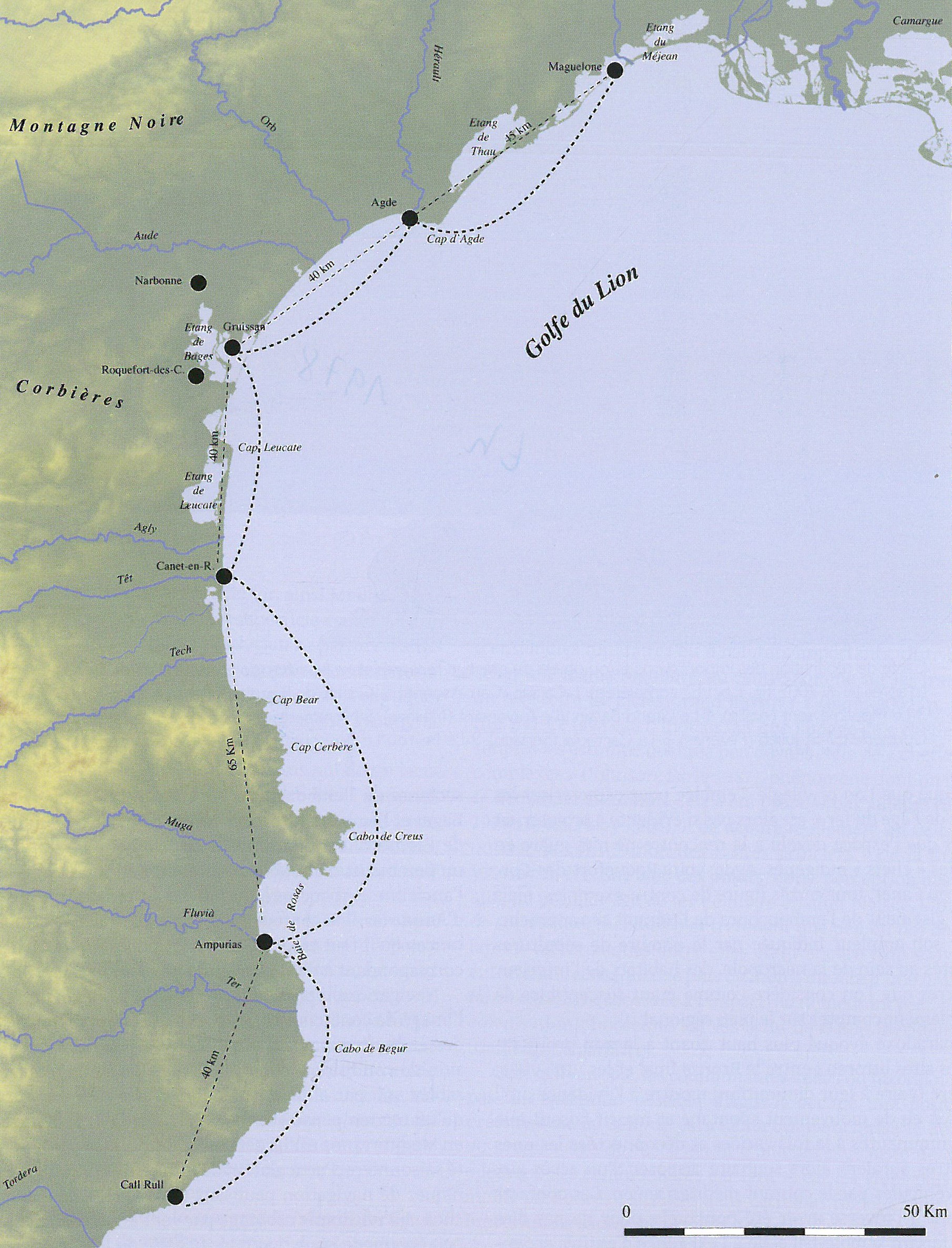
Main emporions in the Gulf of Lion, NW Mediterranean (Gailledrat 2005)
During the same period (6th c. BC) coastal trading posts installed almost systematically at the mouth of river valleys and approximately 40 km from each other (1 day’s cabotage)
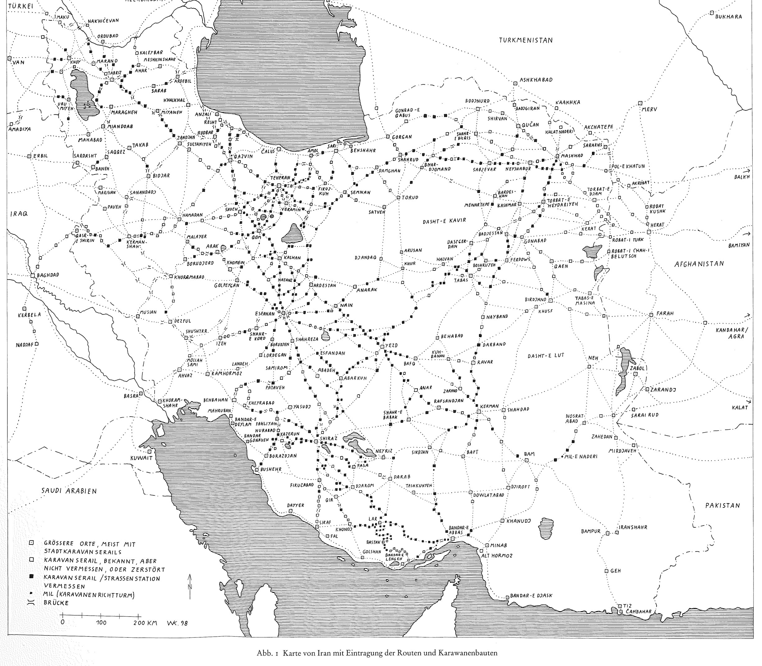
Caravanserais in Iran (Kleiss 1996 )
During the Late Islamic period (15th-18th c. AD) trade posts (caravanserais) have been build along trading roads. They are close to water sources and separated from each other by about 20-30 km (1 day’s transport).

Gradient pattern

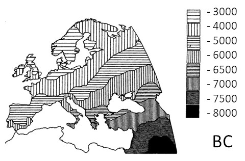
Ammerman and Cavalli-Sforza, 1971, Measuring the rate of spread of early farming in Europe
Diffusion (spatial and temporal). In the case of a linear gradient, the calculation of the centroid of a group of points is a good indicator of its evolution.

2-dim data shape

3-dim data

3-dim or more data

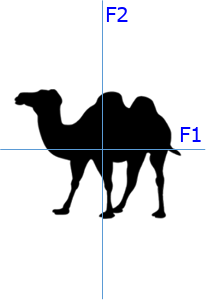
Factorial Analysis (FA)

➡️
Factorial Analysis is the generic term for multivariate (or multifactorial) analysis

3-dim or more data

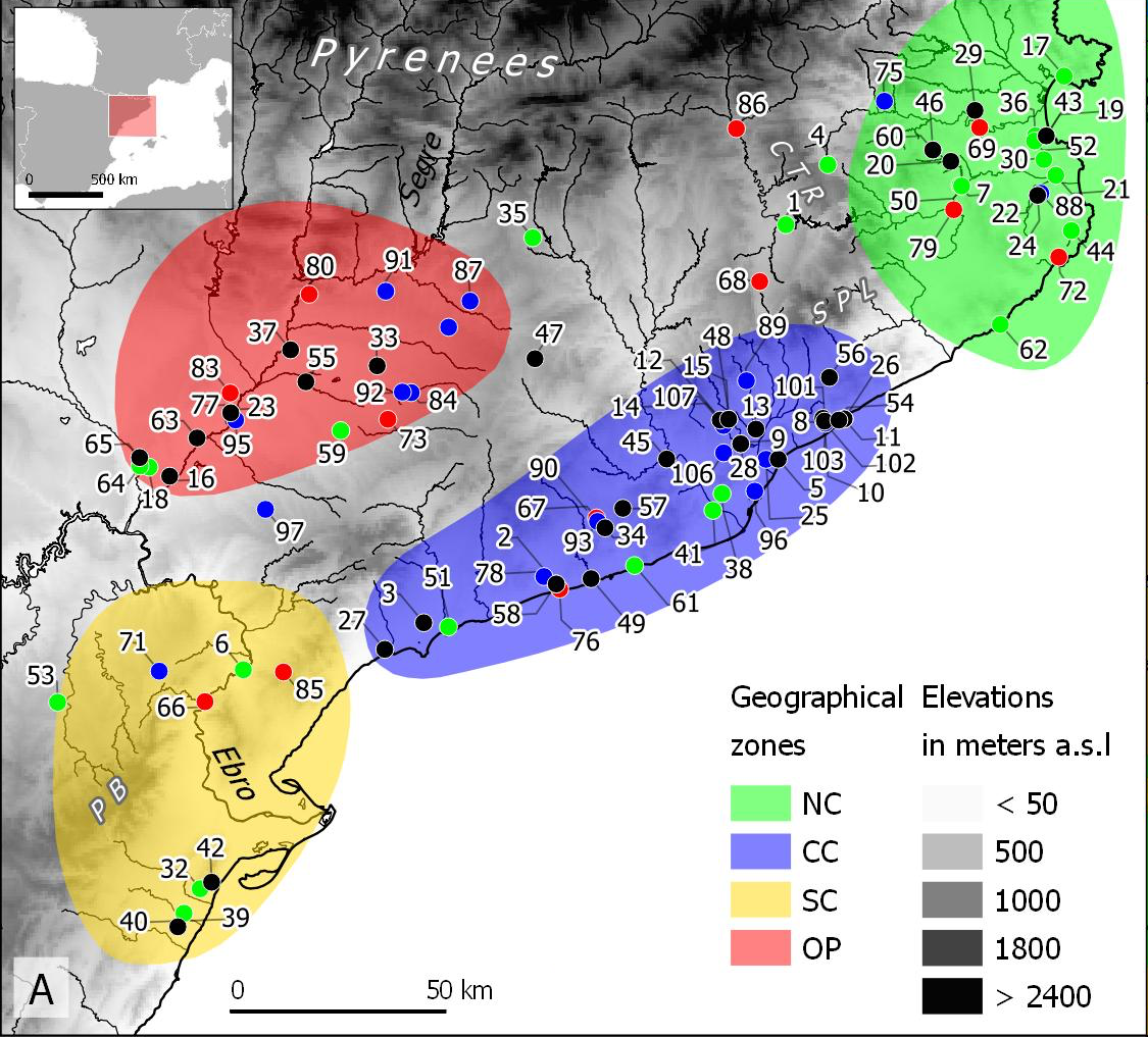
Map of NE Iberia with locations of the studied sites
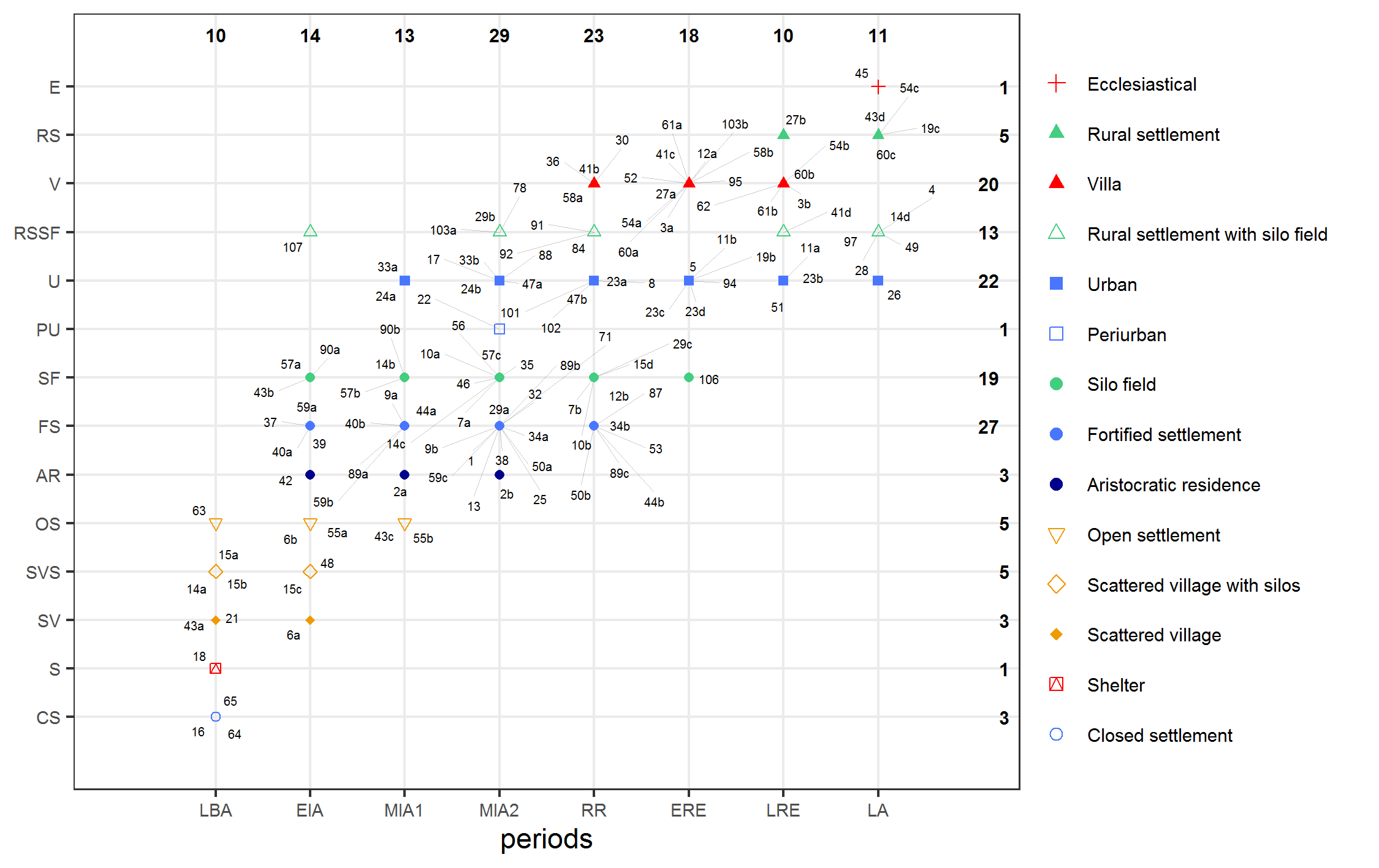
Chrono-typology seriation of the 127 studied assemblages from Late Bronze Age to Late Antiquity
Correspondence Analysis (CA)

\(\ge\) 2 rows, \(\ge\) 2 columns, \(\emptyset\) missing data, \(\emptyset\) negative values, \(\forall\) data with the same scale
CA of sites’ NISP profiles during the LBA
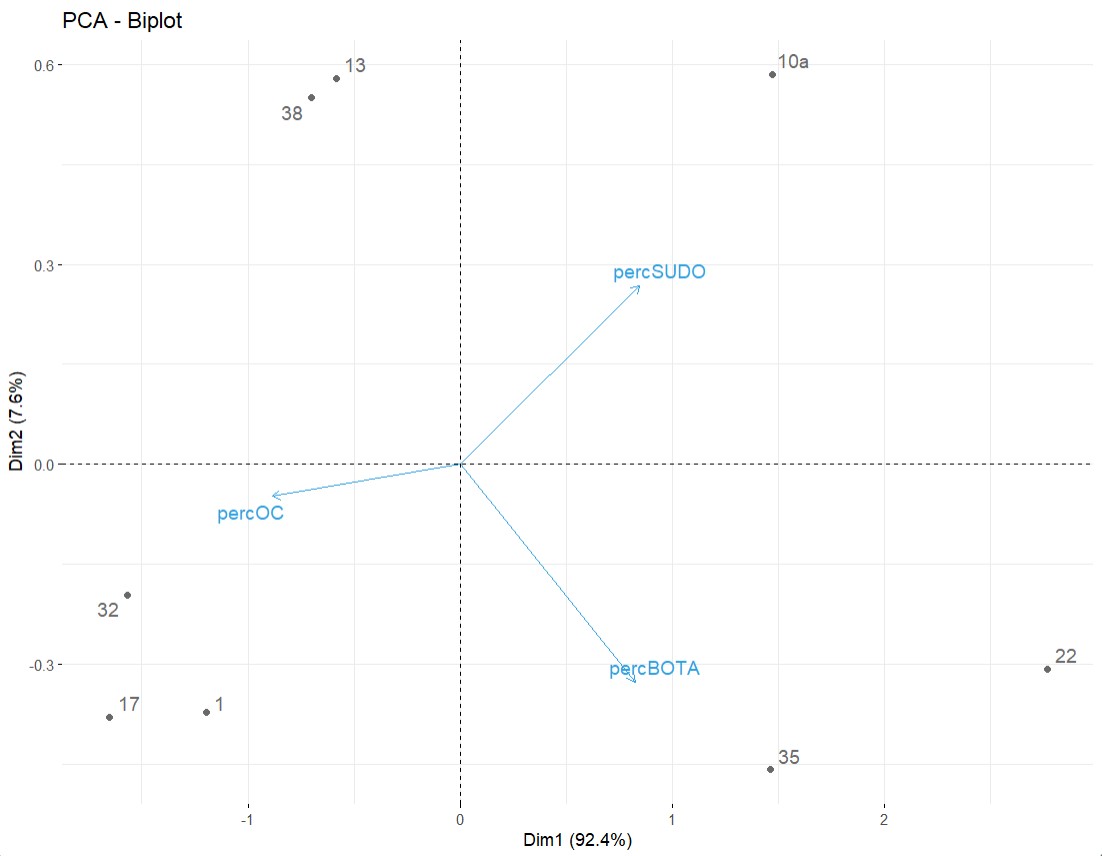
Principal Component Analysis (PCA)

quantitative data, \(\ge\) 3 rows, \(\ge\) 3 columns, nb rows \(\ge\) 10x nb of columns
PCA of sites’ NISP profiles during the MIA2
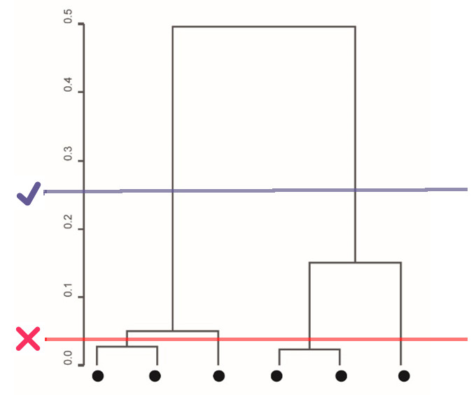
Hierachical Clustering Analysis (HCA)

related to CA, PCA or MFA
HCA of sites’ NISP profiles during the LBA
Linear Discriminant Analysis (LDA)

sensitive to outliers, the size of the smallest group must be larger than the number of predictor variables
LDA of sites’ NISP profiles during the LBA

Seriation

Practice

Use of the OxfordPots dataset (archdata R package), to reproduce the linear regression of Oxford potteries distribution by Fulford and Hodder7
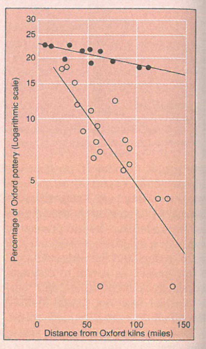
Regression analysis of Late Roman fine ware (Oxford pots) presumably transported by river (black circles) or land (hollow circles)

R code:

install.packages("archdata")
library(archdata)
data("OxfordPots")
OxfordPots$OxfordPct.log <- log(OxfordPots$OxfordPct)
Oxford.water.transport <- subset(OxfordPots, WaterTrans == 1)
Oxford.water.transport.no <- subset(OxfordPots, WaterTrans == 0)
plot(x = Oxford.water.transport$OxfordDst,
     y = Oxford.water.transport$OxfordPct.log,
     xlim = c(0, max(Oxford.water.transport$OxfordDst)),
     ylim = c(0, max(Oxford.water.transport$OxfordPct.log)),
     pch = 16,
     xlab = "Distance from Oxford kilns (miles)", 
     ylab = "Percentage of Oxford pottery (Logarithmic scale)")
points(x = Oxford.water.transport.no$OxfordDst,
       y = Oxford.water.transport.no$OxfordPct.log)
abline(lm(OxfordPct.log ~ OxfordDst, data = Oxford.water.transport))
abline(lm(OxfordPct.log ~ OxfordDst, data = Oxford.water.transport.no))

https://github.com/zoometh/thomashuet/blob/main/teach/stats/stats/dim2/regression-basic.R


Bibliographic resources

Renfrew, C., & Bahn, P. (2012). Archaeology: theories, methods and practice. Thames and Hudson.
Djindjian, F., & Gardin, J. C. (1991). Méthodes pour l’archéologie. Paris: A. Colin.
Chenorkian R. (1996). Pratique archéologique statistique et graphique. Paris: Errance et Adam.
Barceló, J. A. (2007). Introducción al estudio de la variabilidad de las evidencias arqueológicas. Bellaterra: Universitat Autònoma de Barcelona.

Contact

Footnotes

  1. i.e. Post-positivism

  2. Findable, Accessible, Reusable, Interoperable

  3. i.e. goodness-of-fit

  4. “Sociological theory, if it is to advance significantly, must proceed on these interconnected planes: (1) by developing special theories from which to derive hypotheses that can be empirically investigated and (2) by evolving a progressively more general conceptual scheme that is adequate to consolidate groups of special theories” Robert K. Merton, 1968

  5. An archaeological culture is a polythetic assemblage of features more frequently associated with each other within a given area than outside it (Clarke 1968, Brun 1988, Shennan et al. 2015, etc.)

  6. “people think closer things are more similar”, Montello et Fabrikant, 2006.

  7. Fulford, M. G., & Hodder, I. (1974). A regression analysis of some Late Romano-British pottery: a case study. Oxoniensia, 39, 26-33.